This is the tutorial for the paper “Missing data in TBI research: A five step approach for multiple imputation”.
Step 1 - Exploration
For the quantity and patterns of missingness
VIM::aggr(dti)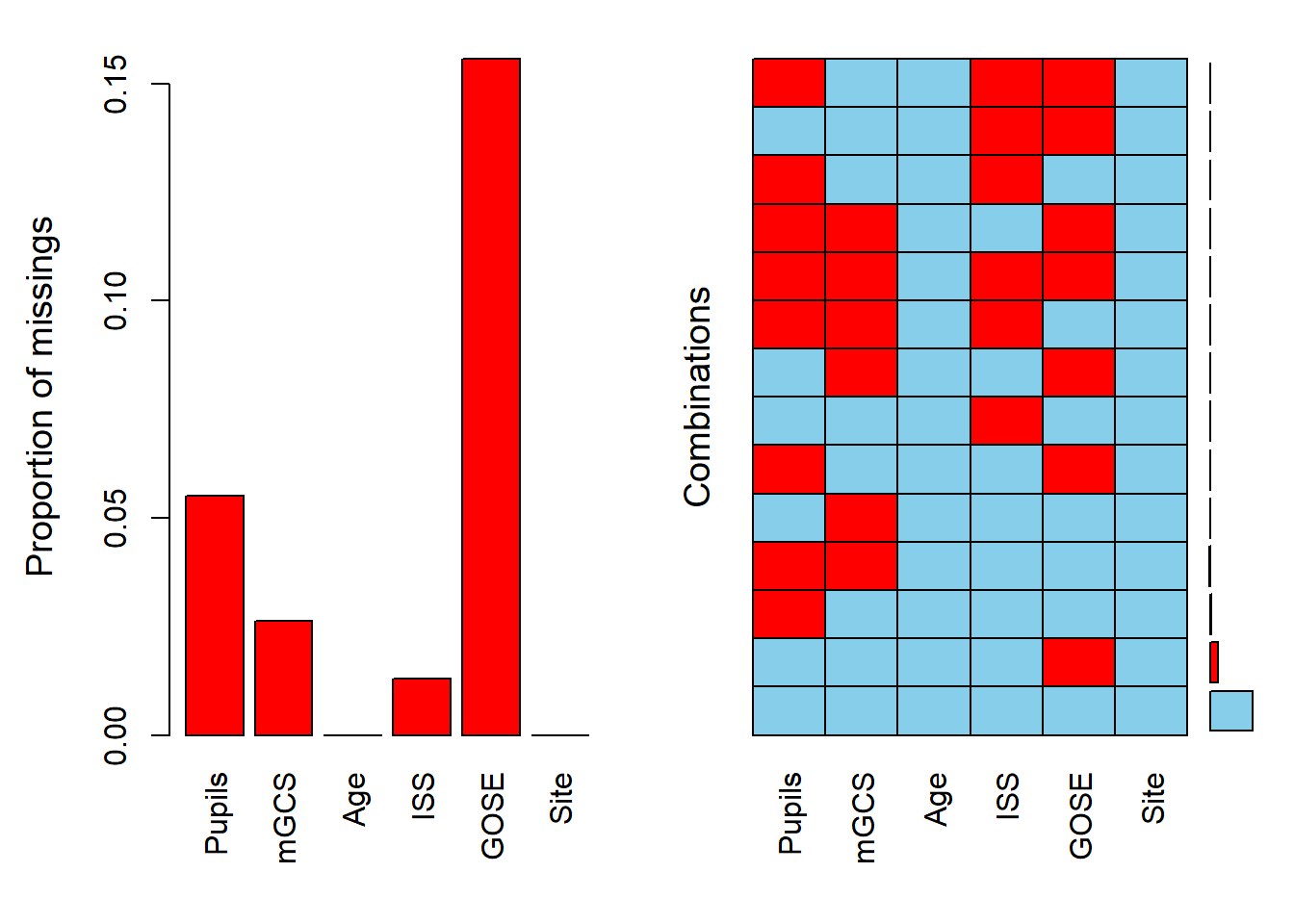
For the correlation between variables
corr <- cor(sapply(dti, as.numeric), use = "pairwise.complete.obs", method = "spearman")
corrplot::corrplot(corr, type = "lower")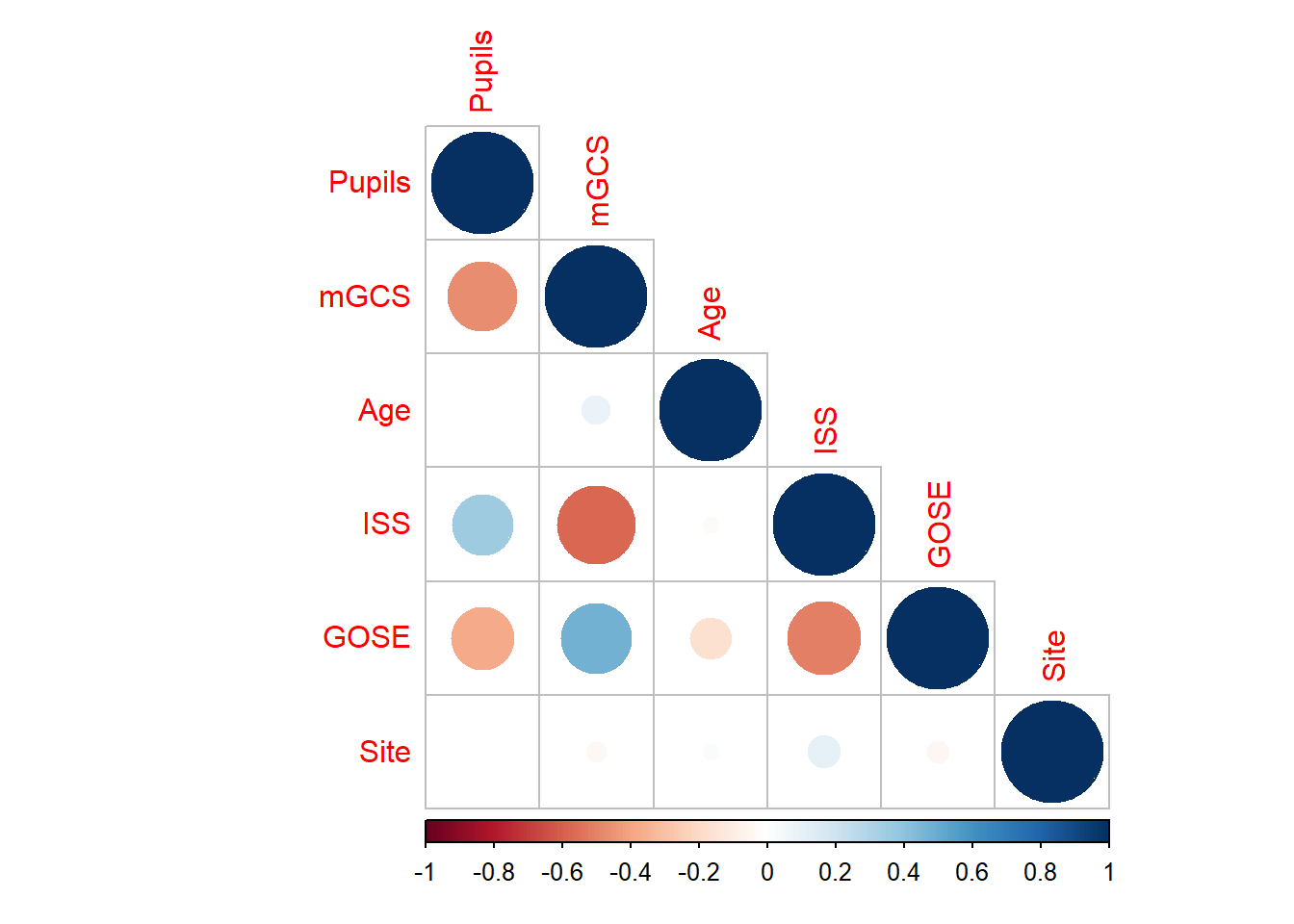
For overall distributions and % missingess
# The first time:
# library(devtools)
# install_github("bgravesteijn/bgravesteijn")
bgravesteijn::distr.na(dti)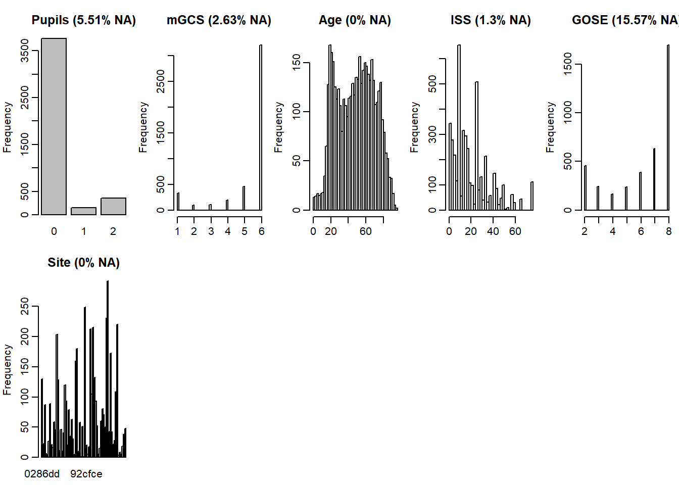
To test MAR
summary(glm(I(is.na(Pupils))~mGCS+Age+ISS+GOSE, data=dti, family="binomial"))##
## Call:
## glm(formula = I(is.na(Pupils)) ~ mGCS + Age + ISS + GOSE, family = "binomial",
## data = dti)
##
## Deviance Residuals:
## Min 1Q Median 3Q Max
## -0.3502 -0.2998 -0.2797 -0.2559 2.8021
##
## Coefficients:
## Estimate Std. Error z value Pr(>|z|)
## (Intercept) -3.284e+00 6.052e-01 -5.427 5.74e-08 ***
## mGCS -3.960e-03 7.834e-02 -0.051 0.960
## Age 6.136e-03 4.244e-03 1.446 0.148
## ISS -1.085e-02 6.992e-03 -1.552 0.121
## GOSE 9.707e-07 5.064e-02 0.000 1.000
## ---
## Signif. codes: 0 '***' 0.001 '**' 0.01 '*' 0.05 '.' 0.1 ' ' 1
##
## (Dispersion parameter for binomial family taken to be 1)
##
## Null deviance: 1210.7 on 3698 degrees of freedom
## Residual deviance: 1204.2 on 3694 degrees of freedom
## (823 observations deleted due to missingness)
## AIC: 1214.2
##
## Number of Fisher Scoring iterations: 6summary(glm(I(is.na(mGCS))~Pupils+Age+ISS+GOSE, data=dti, family="binomial"))##
## Call:
## glm(formula = I(is.na(mGCS)) ~ Pupils + Age + ISS + GOSE, family = "binomial",
## data = dti)
##
## Deviance Residuals:
## Min 1Q Median 3Q Max
## -0.3886 -0.1504 -0.1199 -0.0959 3.3980
##
## Coefficients:
## Estimate Std. Error z value Pr(>|z|)
## (Intercept) -2.251663 0.919995 -2.447 0.01439 *
## Pupils1 0.236735 0.646505 0.366 0.71423
## Pupils2 -1.372729 0.787067 -1.744 0.08114 .
## Age -0.016638 0.008650 -1.924 0.05440 .
## ISS 0.005061 0.011033 0.459 0.64644
## GOSE -0.288974 0.093874 -3.078 0.00208 **
## ---
## Signif. codes: 0 '***' 0.001 '**' 0.01 '*' 0.05 '.' 0.1 ' ' 1
##
## (Dispersion parameter for binomial family taken to be 1)
##
## Null deviance: 384.53 on 3589 degrees of freedom
## Residual deviance: 368.39 on 3584 degrees of freedom
## (932 observations deleted due to missingness)
## AIC: 380.39
##
## Number of Fisher Scoring iterations: 8summary(glm(I(is.na(ISS))~mGCS+Age+Pupils+GOSE, data=dti, family="binomial"))##
## Call:
## glm(formula = I(is.na(ISS)) ~ mGCS + Age + Pupils + GOSE, family = "binomial",
## data = dti)
##
## Deviance Residuals:
## Min 1Q Median 3Q Max
## -0.1677 -0.1266 -0.1213 -0.1150 3.4560
##
## Coefficients:
## Estimate Std. Error z value Pr(>|z|)
## (Intercept) -5.295091 1.212123 -4.368 1.25e-05 ***
## mGCS 0.146638 0.193995 0.756 0.450
## Age 0.002723 0.009820 0.277 0.782
## Pupils1 0.072399 1.065004 0.068 0.946
## Pupils2 -0.800449 1.107279 -0.723 0.470
## GOSE -0.081076 0.107459 -0.754 0.451
## ---
## Signif. codes: 0 '***' 0.001 '**' 0.01 '*' 0.05 '.' 0.1 ' ' 1
##
## (Dispersion parameter for binomial family taken to be 1)
##
## Null deviance: 307.94 on 3581 degrees of freedom
## Residual deviance: 305.70 on 3576 degrees of freedom
## (940 observations deleted due to missingness)
## AIC: 317.7
##
## Number of Fisher Scoring iterations: 8summary(glm(I(is.na(GOSE))~mGCS+Age+ISS+Pupils, data=dti, family="binomial"))##
## Call:
## glm(formula = I(is.na(GOSE)) ~ mGCS + Age + ISS + Pupils, family = "binomial",
## data = dti)
##
## Deviance Residuals:
## Min 1Q Median 3Q Max
## -0.6931 -0.6144 -0.5683 -0.4778 2.3585
##
## Coefficients:
## Estimate Std. Error z value Pr(>|z|)
## (Intercept) -1.308427 0.278584 -4.697 2.64e-06 ***
## mGCS 0.008975 0.041375 0.217 0.828279
## Age -0.003581 0.002023 -1.771 0.076622 .
## ISS -0.013434 0.003480 -3.860 0.000113 ***
## Pupils1 0.048037 0.254093 0.189 0.850051
## Pupils2 -0.309961 0.212622 -1.458 0.144895
## ---
## Signif. codes: 0 '***' 0.001 '**' 0.01 '*' 0.05 '.' 0.1 ' ' 1
##
## (Dispersion parameter for binomial family taken to be 1)
##
## Null deviance: 3580.2 on 4194 degrees of freedom
## Residual deviance: 3543.4 on 4189 degrees of freedom
## (327 observations deleted due to missingness)
## AIC: 3555.4
##
## Number of Fisher Scoring iterations: 4Step 3 - Imputation
Multiple - single level
library(mice)

miceimp <- dti

miceimp0 <- mice(miceimp, maxit=0)

meth <- miceimp0$method
pred <- miceimp0$predictorMatrix

meth[which(meth=="pmm")] <- "midastouch" #the improved version of PMM, of the miceadds package

pred[, "Site"] <- 0 #don't use sitecode to impute

miceimp <- mice(data = miceimp, method = meth, predictorMatrix = pred, m=5, printFlag = FALSE, set.seed=1234)
Multiple - multilevel
library(jomo)

jomoimp <- dti

jomoimp$GOSE <- factor(jomoimp$GOSE, ordered=TRUE)

# specify the level of each variable
lvl <- c(GOSE=1,
         Pupils = 1,
         mGCS = 1,
         Age = 1,
         ISS = 1,
         Site = 2)

jomoimp <- data.frame(jomoimp) #so the subsetting within the function works

fml <- as.formula("GOSE~Pupils+mGCS+Age+ISS+(1|Site)")

jomo.chain <- jomo.clmm.MCMCchain(fml,data = jomoimp[,names(lvl)], level=lvl)

jomoimp <- jomo.clmm(fml,data = jomoimp[,names(lvl)], level=lvl, nimp = 5)

jomoimp.2 <- datalist2mids(split(jomoimp,
                                 jomoimp$Imputation)[-1])
Step 4 - Diagnostics
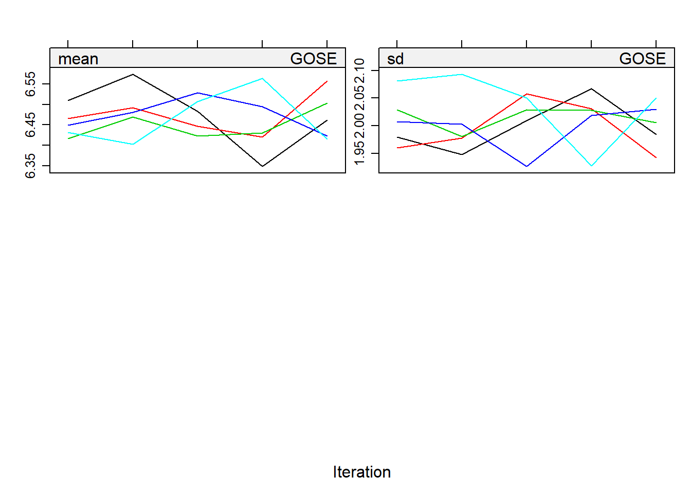
print("MICE")## [1] "MICE"plot(miceimp)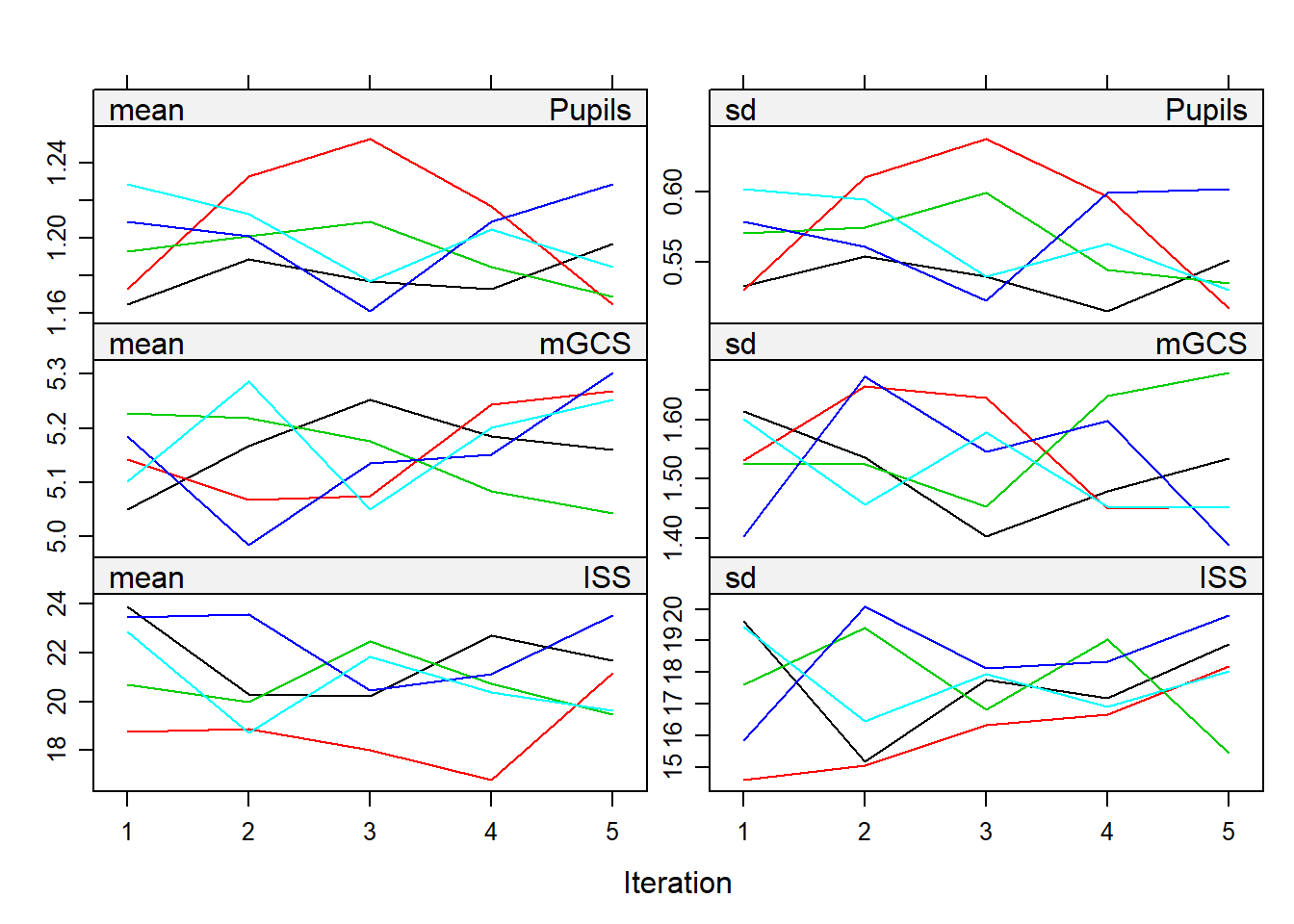
bgravesteijn::distr.na(complete(miceimp,1))
densityplot(miceimp)
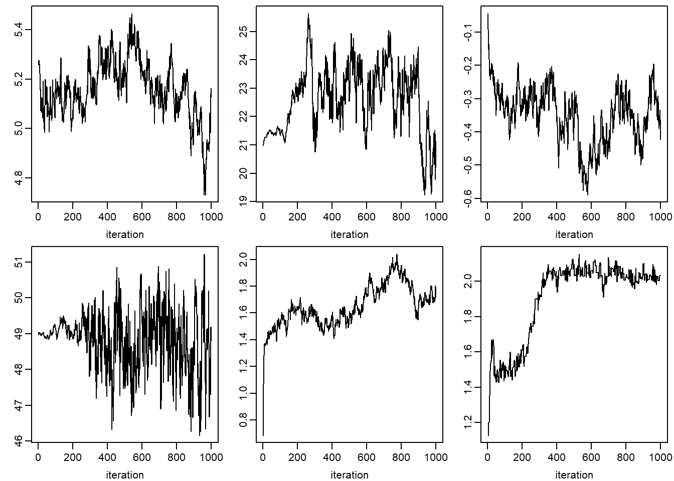
print("JOMO")## [1] "JOMO"par(mfcol = c(2, 3), mar = c(3, 2.5, 0.5, 0.5), mgp = c(2, 0.6, 0))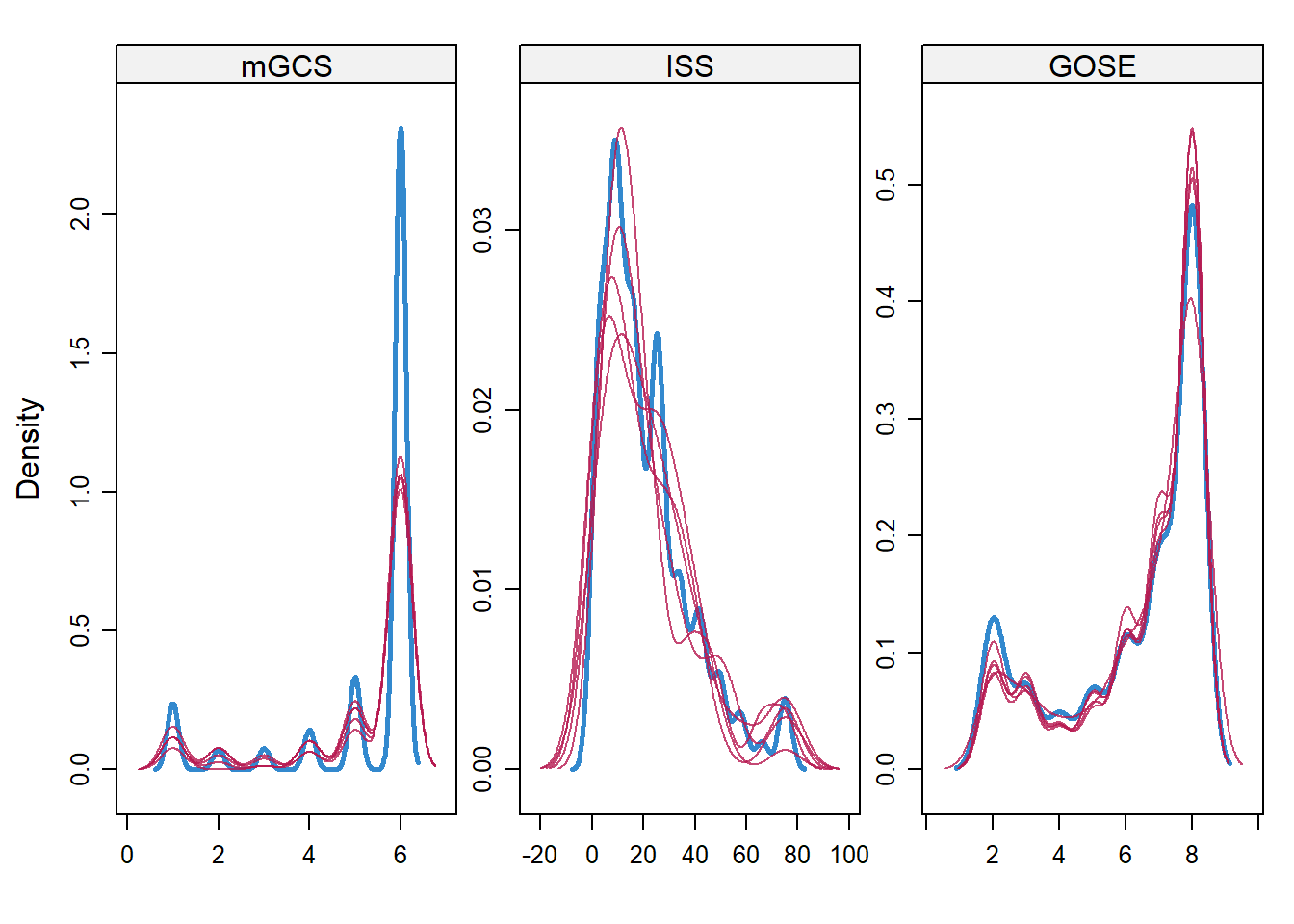
apply(jomo.chain$collectbeta[1, ,], 1, plot, type = "l",
      xlab = 'iteration', ylab = '')
## NULLfor (k in 1:dim(jomo.chain$collectomega)[1]) {
apply(jomo.chain$collectomega[k, , ], 1, plot, type = "l",
xlab = 'iteration', ylab = '')
}
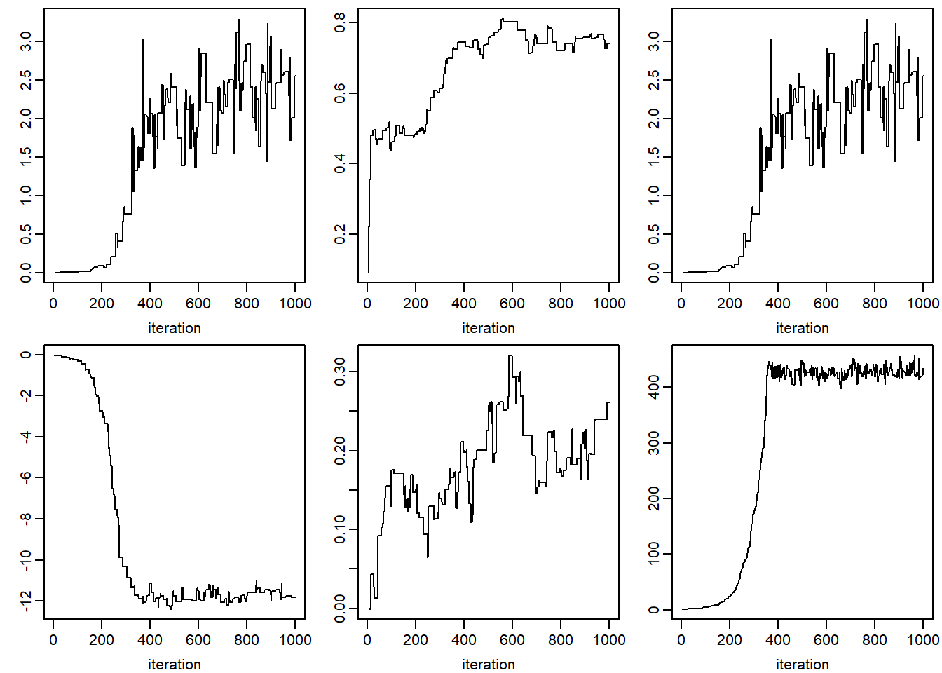
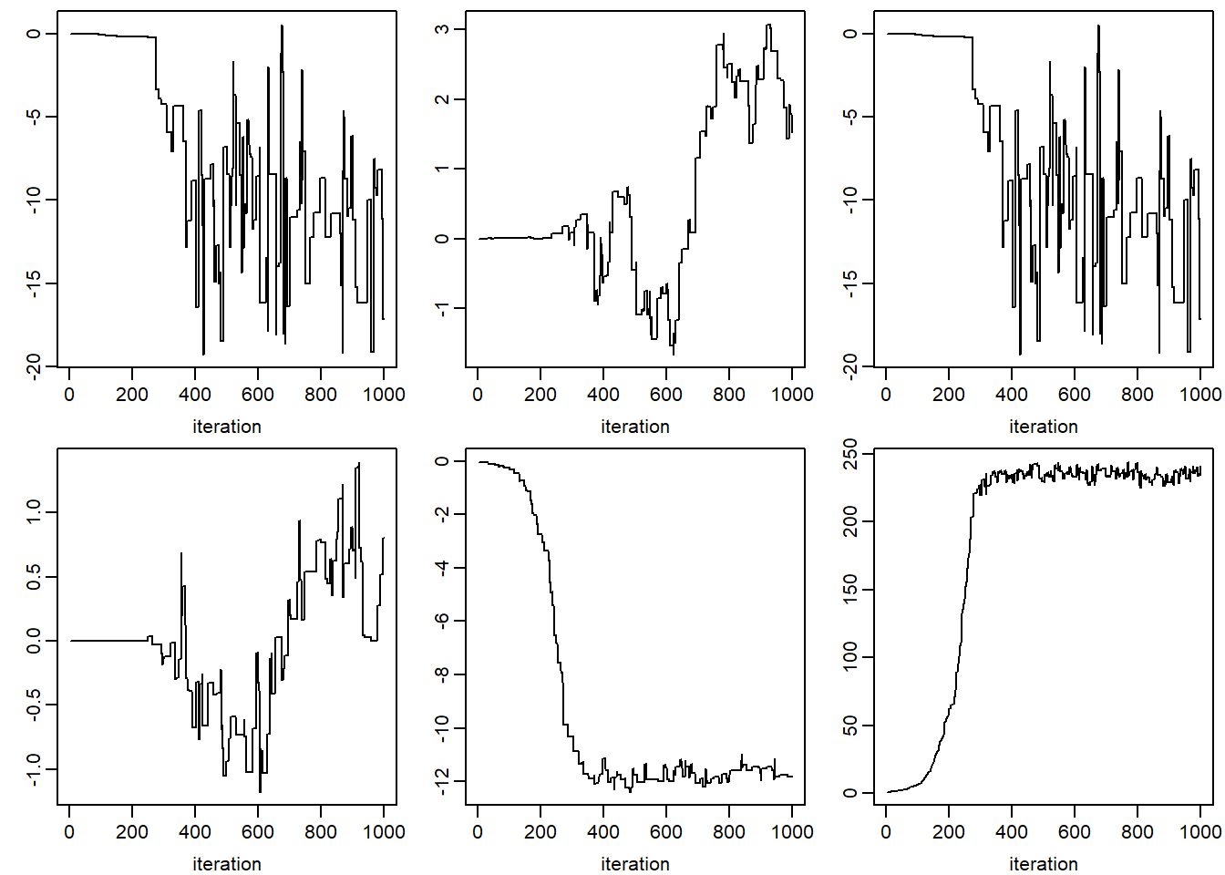
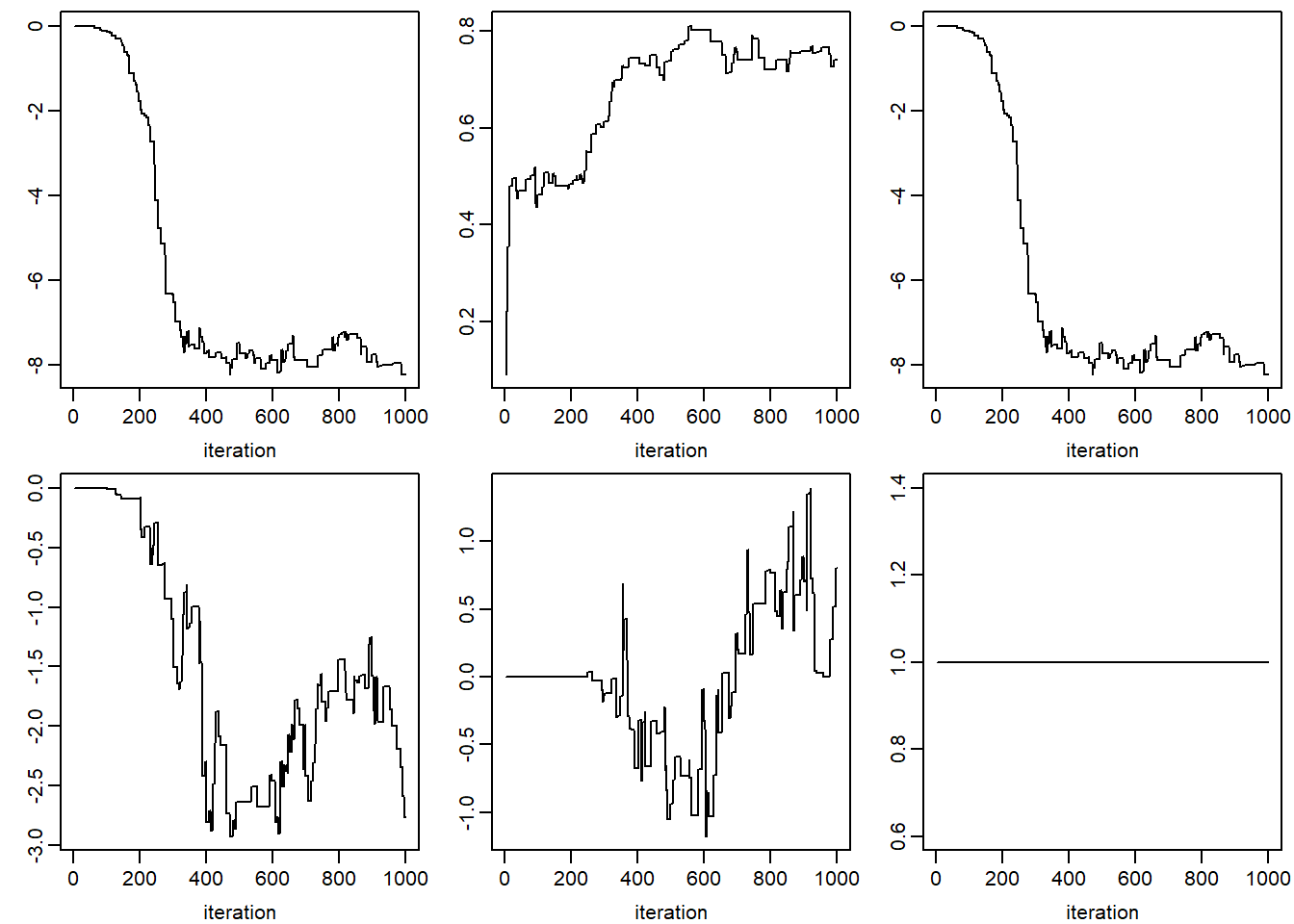
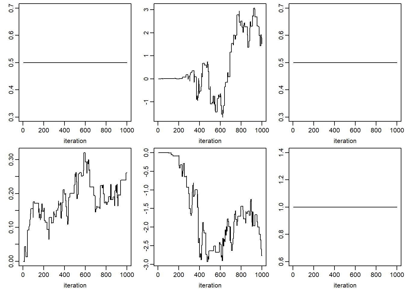
apply(jomo.chain$collectbetaY[1, ,], 1, plot, type = "l",
      xlab = 'iteration', ylab = '')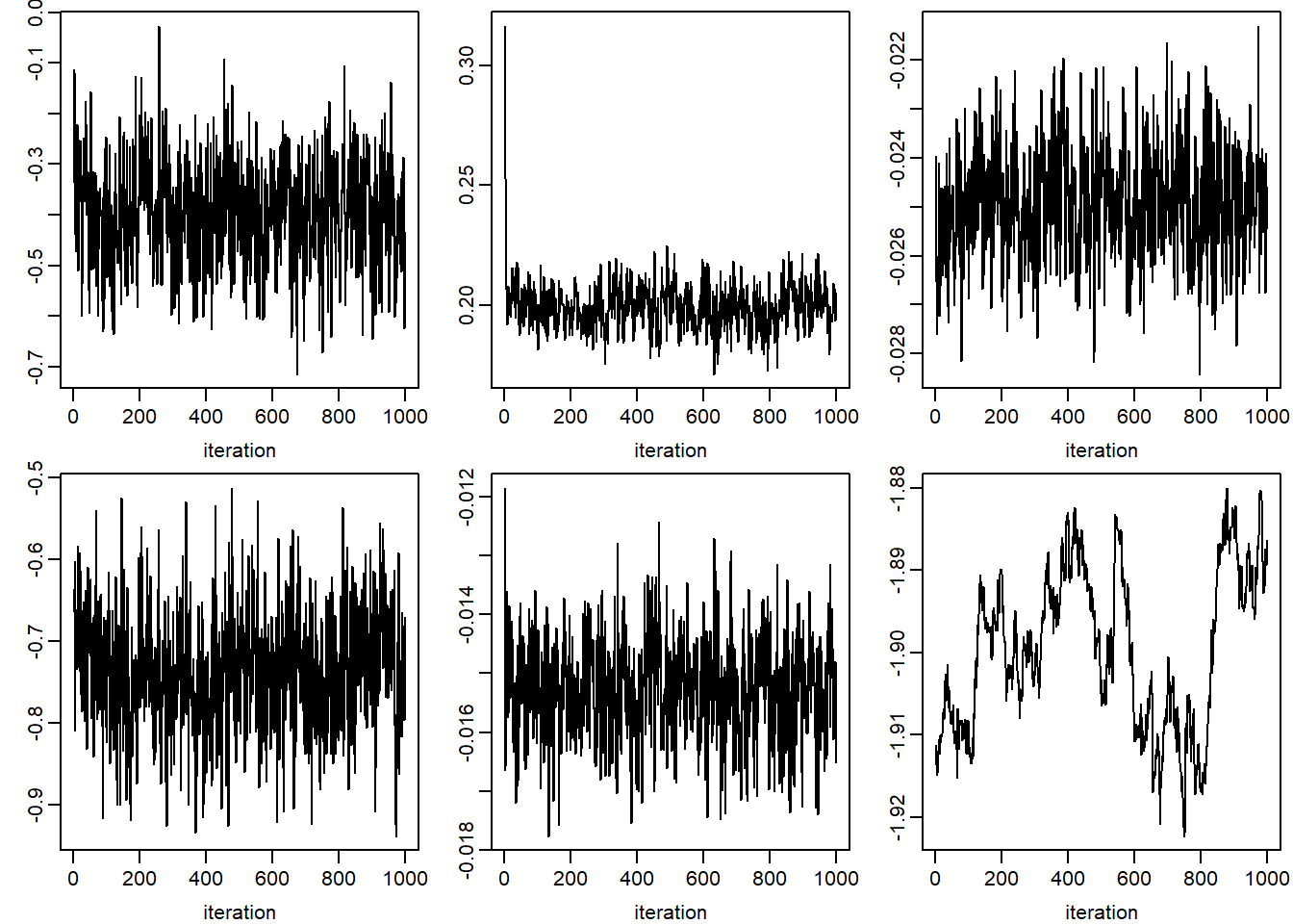
## NULLplot(jomo.chain$collectvarY, type = 'l')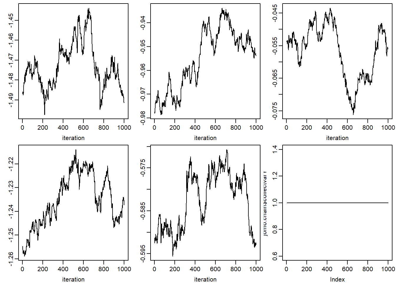
bgravesteijn::distr.na(complete(jomoimp.2,1))
densityplot(jomoimp.2)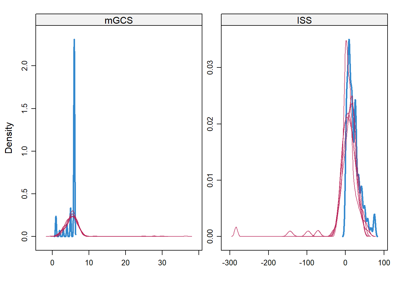
Step 5 - Fitting
library(rms)
fit2 <- fit.mult.impute(GOSE~mGCS+Age+Pupils, fitter=lrm, xtrans = miceimp, data=dti)
##
## Variance Inflation Factors Due to Imputation:
##
## y>=3 y>=4 y>=5 y>=6 y>=7 y>=8 mGCS Age
## 1.35 1.38 1.35 1.36 1.38 1.49 1.20 1.30
## Pupils=1 Pupils=2
## 1.10 1.19
##
## Rate of Missing Information:
##
## y>=3 y>=4 y>=5 y>=6 y>=7 y>=8 mGCS Age
## 0.26 0.27 0.26 0.26 0.28 0.33 0.16 0.23
## Pupils=1 Pupils=2
## 0.09 0.16
##
## d.f. for t-distribution for Tests of Single Coefficients:
##
## y>=3 y>=4 y>=5 y>=6 y>=7 y>=8 mGCS Age
## 58.86 53.56 60.35 57.13 52.56 37.41 150.10 73.84
## Pupils=1 Pupils=2
## 486.50 163.26
##
## The following fit components were averaged over the 5 model fits:
##
## stats linear.predictorsfit2## Logistic Regression Model
##
## fit.mult.impute(formula = GOSE ~ mGCS + Age + Pupils, fitter = lrm,
## xtrans = miceimp, data = dti)
##
##
## Frequencies of Responses
##
## 2 3 4 5 6 7 8
## 521 292 192 272 464 745 2036
##
## Model Likelihood Discrimination Rank Discrim.
## Ratio Test Indexes Indexes
## Obs 4522 LR chi2 1464.45 R2 0.288 C 0.703
## max |deriv| 1e-09 d.f. 4 g 1.173 Dxy 0.406
## Pr(> chi2) <0.0001 gr 3.233 gamma 0.408
## gp 0.194 tau-a 0.299
## Brier 0.120
##
## Coef S.E. Wald Z Pr(>|Z|)
## y>=3 0.8848 0.1580 5.60 <0.0001
## y>=4 0.1476 0.1575 0.94 0.3486
## y>=5 -0.2216 0.1559 -1.42 0.1552
## y>=6 -0.6654 0.1573 -4.23 <0.0001
## y>=7 -1.2672 0.1602 -7.91 <0.0001
## y>=8 -2.0792 0.1686 -12.33 <0.0001
## mGCS 0.5453 0.0247 22.05 <0.0001
## Age -0.0209 0.0016 -13.05 <0.0001
## Pupils=1 -0.9522 0.1555 -6.13 <0.0001
## Pupils=2 -1.5360 0.1273 -12.07 <0.0001
##